cs1120 Problem Set 3:
Limning L-System Fractals

Collaboration Policy - Read Carefully

Before starting to work with a partner, you should go through questions 1 and 2 yourself on paper. When you meet with your partner (if any), check if you made the same predictions. If there are any discrepancies, try to decide which is correct before using Python to evaluate the expressions.

If you have a partner, you and your partner should work together on the rest of the assignment. You should read the whole problem set yourself and think about the questions before beginning to work on them with your partner. Both partners need to understand everything you submit.

Remember to follow the pledge you read and signed at the beginning of the semester. For this assignment, you may consult any outside resources, including books, papers, web sites and people, you wish except for materials from previous cs1120, cs150, and cs200 courses. You may consult an outside person (e.g., another friend who is a CS major but is not in this class) who is not a member of the course staff, but that person cannot type anything in for you and all work must remain your own. That is, you can ask general questions such as "can you explain recursion to me?" or "how do lists work in Python?", but outside sources should never give you specific answers to problem set questions. If you use resources other than the class materials, lectures and course staff, explain what you used in your turn-in.

You are strongly encouraged to take advantage of the scheduled help hours and office hours for this course.

Purpose

• Practice programming with recursive definitions and procedures
• Explore the power of rewrite rules
• Write recursive functions that manipulate lists
• Make a cs1120 course logo better than "The Great Lambda Tree of Infinite Knowledge and Ultimate Power"

Background

In this problem set, you will explore a method of creating fractals known as the Lindenmayer system (or L-system). Aristid Lindemayer, a theoretical biologist at the University of Utrecht, developed the L-system in 1968 as a mathematical theory of plant development. In the late 1980s, he collaborated with Przemyslaw Prusinkiewicz, a computer scientist at the University of Regina, to explore computational properties of the L-system and developed many of the ideas on which this problem set is based.

The idea behind L-system fractals is that we can describe a curve as a list of lines and turns, and create new curves by rewriting old curves. Everything in an L-system curve is either a forward line (denoted by F), or a right turn (denoted by Ra where a is an angle in degrees clockwise). We can denote left turns by using negative angles.

We create fractals by recursively replacing all forward lines in a curve list with the original curve list. Lindemayer found that many objects in nature could be described using regularly repeating patterns. For example, the way some tree branches sprout from a trunk can be described using the pattern: F O(R30 F) F O(R-60 F) F. This is interpreted as: the trunk goes up one unit distance, a branch sprouts at an angle 30 degrees to the trunk and grows for one unit. The O means an offshoot — we draw the curve in the following parentheses, and then return to where we started before the offshoot. The trunk grows another unit and now another branch, this time at -60 degrees relative to the trunk grows for one units. Finally the trunk grows for one more unit. The branches continue to sprout in this manner as they get smaller and smaller, and eventually we reach the leaves.

We can describe this process using replacement rules:

Start: [F]
Rule: F ::= [F O[R30 F] F O[R-60 F] F]

Iteration 0: [F]
Iteration 1: [F O[R30 F] F O[R-60 F] F]
Iteration 2: [F O[R30 F] F O[R-60 F] F O[R30 F O[R30 F] F O[R-60 F] F] F O[R30 F] F O[R-60 F] F O[R-60 F O[R30 F] F O[R-60 F] F] F O[R30 F] F O[R-60 F] F]

Here's what that looks like:

Iteration 0 Iteration 1 Iteration 2 Iteration 5

Iteration 5 (with color) The Great Lambda Tree of Infinite Knowledge and Ultimate Power

Note that L-system command rewriting is similar to the replacement rules in a BNF grammar. The important difference is that with L-system rewriting, each iteration replaces all instances of F in the initial string instead of just picking one to replace.

We can divide the problem of producing an L-system fractal into two main parts:

1. Produce a list of L-system commands that represents the fractal by rewriting according to the L-system rule; and
2. Drawing a list of L-system commands.

Representing L-System Commands

Here is a BNF grammar for L-system commands:

1. CommandSequence ::= [ CommandList ]
   
2. CommandList ::= Command   CommandList
   
3. CommandList ::=
   
4. Command ::= F
   
5. Command ::= RAngle
   
6. Command ::= O CommandSequence
   
7. Angle ::= Number
   

We need to find a way to turn strings in this grammar into lists and objects we can manipulate in a Python program. We will use a list of lists to represent a CommandList and a list of strings to represent different commands. For example, the list ['F'] will denote forward, ['R', angle] will denote a rotation, and ['O', CommandList] will denote an offshoot.

# Command ::= F
def make_forward_command():
	return ['F'] # creates a list of one element, 'F'

# Command ::= R Angle
def make_rotate_command(angle): 
	return ['R', angle] # creates a list of two elements, 'R' and a number

# Command ::= O CommandSequence
def make_offshoot_command(commandsequence): 
	return ['O', commandsequence] # creates a list of two elements, 'O' and another list 

>>> is_forward(make_forward_command())
True
>>> is_forward(make_rotate_command(90))
False
>>> get_angle(make_rotate_command(90))
90
>>> get_angle(make_forward_command())
# ERROR

New Python Special Forms

New Python Syntax: elif

if letter == 'G':
        return 'C'
elif letter == 'C':
        return 'G'
elif letter == 'A':
        return 'T'
else:   # must be 'T' 
        return 'A'

New Python Concept: Global Variables

By contrast, a global variable is a variable that lives outside of any function and can be referenced anywhere in the program. Python has a special way to do this, but using global variables is typically considered bad programming practice (i.e., "bad style" or "ugly"). You should not use global variables but you should know that they exist and how they work.

my_variable = 5 # Initialize a global variable.
                # Note that this variable is defined
                # outside of the body of any function.

def change_the_value_of_my_variable(x):
        # We must tell Python that we want access to our global variable.
        # This next line, starting with the keyword syntax "global",
        # does just that. 
        global my_variable 
        # Now we if we assign a new value to our global variable, that
        # assignment will live on even after this function finishes. 
        my_variable = x

def common_bug(x):
        # If we forget to say "global", Python will instead make a
        # new local variable that just happens to have the same name!
        my_variable = x 
        # The above assignment does not change our global variable.

print(my_variable)
change_the_value_of_my_variable(7)
print(my_variable)
common_bug(10)
print(my_variable)

New Python Concept: Functions nested within other functions

>>> square = lambda(t) : t * t
>>> print square(5) 
25

>>> def make_adder(a):
           return lambda(b) : a + b
>>> add_three = make_adder(3)
>>> print add_three(4)
7
>>> print add_three(-2)
1

>>> def make_adder(a):
           def adder(b):
                return a + b
           return adder
>>> add_three = make_adder(3)
>>> print add_three(4)
7
>>> print add_three(-2)
1
>>> print adder(3)
# ERROR: adder is not visible at the outermost level.
# You can only refer to it by name inside of make_adder!

While lambda is very convenient, Python will not allow us to put more than one line of code in the body of a lambda — for example, you may have noticed that lambda implicitly returns its body, so you can't use our usual if statement inside a lambda. Nested functions allow us to write more complicated code such as loops and conditional statements. In the code for this problem set, graphics.py has many examples of nested functions.

Having introduced these three new Python concepts, we now have everything we need to get back to drawing fractals!

Rewriting Curves

Start: [F]
Rule: [F] ::= [[F], [O, [[R, 30], [F]]], [F], [O, [[R,60], [F]], [F]]]

So, for every command in the list:

• If the command is an F command, replace it with the replacement commands
• If the command is an RAngle command, keep it unchanged
• If the command is an OCommandSequence command, recursively rewrite every command in the offshoot's command list the same way

For example, consider a simple L-System rewriting:

Start: [F]
Rule: [F] ::= [[F], [R, 30], [F]]

Iteration1: [[F], [R, 30], [F]]
Iteration2: [[F], [R, 30], [F], [R, 30], [F], [R, 30], [F]]

Iteration1: [[[F], [R, 30], [F]]]
Iteration2: [[[F], [R, 30], [F]], [R, 30], [[F], [R, 30], [F]]]

def flatten_commands(ll):
    if len(ll) == 0:
        return ll
    elif is_lsystem_command(ll[0]):
        return [ll[0]] + flatten_commands(ll[1:])
    else:
        x = [flatten_commands(ll[0])] + flatten_commands(ll[1:])
        return x[0] + x[1:]

If you define these procedures correctly, you should produce these evaluations:

>>> rewrite_lcommands(['F'], [['F'],['R', 30], ['F']])
[['F'],['R', 30], ['F']]
>>> rewrite_lcommands([['F'],['R', 30], ['F']], [['F'], ['F'], ['R', 30]])
[['F'], ['F'], ['R', 30], ['R', 30], ['F'], ['F'], ['R', 30]]

To make interesting L-system curves, we will need to apply rewrite_lcommands many times. We will leave that until the last question. Next, we will work on turning sequences of L-system commands into curves we can draw.

Drawing L-System Fractals

You can think of the number between 0 and 1 as time — the first point of the curve you draw will be the point returned by curve(0.0), the middle part of the curve you draw will be the point returned by curve(0.5), and the last part of the curve you draw will be the point returned by curve(1.0).

Of course, we can't really evaluate the curve function at every value between 0 and 1 (because there are infinitely many of them — it would take too long!). Instead, we will evaluate it at a large number of points distributed between 0 and 1 to display an approximation of the curve.

Points

We will use a coordinate system from (0, 0) to (1, 1):

Points have x and y coordinates. To represent points we would like to define procedures make_point, x_of_point and y_of_point. We will use lists to represent points. Our pictures will be more interesting if points can have color too. So, we represent a colored point using a list of three values: x, y and color:

def make_point(x,y):
    return [x,y, (0,0,0)]  # (0,0,0) is the red-green-blue color "black"

def make_colored_point(x,y,c):
    return [x,y,c]

def x_of_point(point):
	return point[0]

def y_of_point(point):
	return point[1]
	
def color_of_point(point):
	return point[2]

We have provided some procedures for drawing on the window in graphics.py:

• window_draw_point(point) — Draw the point on the window. For example, window_draw_point(make_point(0.5, 0.5)) will place a black dot in the center of the window. (The point is only one pixel, so it is hard to see.)
• window_draw_line(point0, point1) — Draw a black line from point0 to point1. For example, window_draw_line(make_point(0.0, 0.0), make_point(1.0, 1.0)) will draw a diagonal line from the bottom left corner to the top right corner.

Read through graphics.py and look for other handy functions.

Drawing Curves

def mid_line(time)
        return make_point(time, 0.5)

Predict what x_of_point(mid_line(0.7)) and y_of_point(mid_line(0.7)) should evaluate to. Try evaluating them in Pycharm.

Of course, there are infinitely many values between 0.0 and 1.0, so we can't apply the curve function to all of them. Instead, we select enough values to show the curve well. To draw a curve, we need to apply the curve procedure to many values in the range from 0.0 to 1.0 and draw each point it evaluates to. Here's a procedure that does that:

def draw_curve_points(curve, n):
        for step in range(n):   # range(n) = [0, 1, 2, ..., n-1] 
                time = 1.0 * step / n 
                window_draw_point(curve(time))

# For exmaple, if n=5, we will draw the curve with time = 
# 0, 0.2, 0.4, 0.6, and 0.8 
# ... which are five times "evenly distributed" between 0.0 and 1.0. 

Manipulating Curves

For example, the procedure rotate_ccw takes a curve and rotates it 90 degrees counter-clockwise by swapping the x and y points:

def rotate_ccw(curve):
    def new_curve(t):
        ct = curve(t)
        return make_point(y_of_point(ct),x_of_point(ct))
    return new_curve

Note that (rotate_ccw c) evaluates to a new curve that is just like the old curve c but rotated. The function rotate_ccw is a procedure that takes a procedure (a curve) and returns a procedure that is a curve. We created a new local variable, ct, and set it to curve(t) so that we didn't have to call curve(t) two times to get both the x- and the y-value at time t.

Predict what draw_curve_points(rotate_ccw(mid_line), 1000) and draw_curve_points(rotate_ccw(rotate_ccw(mid_line)), 1000) will do. Confirm your predictions by trying them in Pycharm.

(You may have just read over that paragraph and not actually done the prediction. The instructions are not just there to waste time: experience suggests that students who do not do them become confused on subsequent Questions and then come back. Thus you can save time by doing them now! If you already did them, great work!)

Here's another example:

def shrink(curve, scale):
    # For example, scale = 0.25 may mean "one-quarter normal size"         
    def new_curve(t):
        ct = curve(t)
        return make_point(scale*x_of_point(ct), scale*y_of_point(ct))
    return new_curve

The shrink procedure doesn't produce quite what we want because in addition to changing the size of the curve, it moves it around. Why does this happen? Try shrinking a few different curves to make sure you understand why the curve moves.

One way to fix this problem is to center our curves around (0,0) and then translate them to the middle of the screen. In mathematics and geometry, translation means moving a shape without rotating or flipping it. That is, to translate a curve is to "slide" it. We can do this by adding or subtracting constants to the points they produce:

def translate(curve, delta_x, delta_y):
    def new_curve(t):
        ct = curve(t)
        return make_colored_point(delta_x+x_of_point(ct), \
                delta_y+y_of_point(ct), color_of_point(ct))
    return new_curve

def horiz_line(t):
        return make_point(t, 0)

mid_line = translate(horiz_line, 0, 0.5) 

Question 6: To check you understand everything so far, define a curve procedure half_line(t) that uses translate, horiz_line and shrink to define a horizontal line half the width of the window that starts in the middle of the display window.

When you are done, draw_curve_points(half_line, 1000) should produce a horizontal line that starts in the middle of the window and extends to the right boundary.

Hint: If you do not see anything when you are drawing a curve, it may be that you haven't yet applied translate and the points are being drawn along the bottom edge of the screen.

In addition to altering the points a curve produces, we can alter a curve by changing the time values it will see. For example,

def first_half(curve):
	return (lambda(time) : curve(time / 2))

Predict what each of these expressions will do:

• draw_curve_points(first_half(mid_line), 1000)
• draw_curve_points(first_half(first_half(mid_line)), 1000)

The provided code includes several other functions that transform curves including:

• scale_x_y(curve, x_scale, y_scale) — evaluates to curve stretched along the x and y axis by using the scale factors given
• scale(curve, scale) — evaluates to curve stretched along the x and y axis by using the same scale factor
• rotate_around_origin(curve, degrees) — evaluates to curve rotated counterclockwise by the given number of degrees.

It is also useful to have curve transforms where curves may be combined. An example is connect_rigidly(curve1, curve2) which evaluates to a curve that consists of curve1 followed by curve2. The starting point of the new curve is the starting point of curve1 and the end point of curve2 is the ending point of the new curve. Here's how connect_rigidly is defined:

def connect_rigidly(curve1, curve2):
        def new_curve(t):
                # We'll split our time between drawing curve1 and
                # drawing curve2. 
                if(t < 0.5):
                        # When we think it's time 0.0 to 0.5, we'll draw
                        # curve1 so that curve1 thinks it's time 0.0 to 1.0.
                        return curve1(2*t)
                else:
                        # When we think it's time 0.5 to 1.0, we'll draw
                        # curve2 so that curve2 thinks it's time 0.0 to
                        # 1.0.
                        return curve2(2*t - 1)
        return new_curve

Predict what draw_curve_points(connect_rigidly(vertical_mid_line, mid_line), 1000) will do. Is there any difference between that and draw_curve_points(connect_rigidly(mid_line, vertical_mid_line), 1000)? Check your predictions in Pycharm.

Distributing t Values

Consider connect_rigidly(A, connect_rigidly(B, C)) — A will get half of the time points and B and C will each get only one quarter of them. (If you're not sure why, take another look at the connect_rigidly code.) That means that B and C will look dotty or grainy compared to A.

This isn't too big a problem when only a few curves are combined; we can just increase the number of points passed to draw_curve_points to have enough points to make a smooth curve. In this problem set, however, you will be drawing fractal curves made up of thousands of connected curves. Just increasing the number of points won't help much, as you'll see in Question 7.

   connect_rigidly(c1, connect_rigidly(c2, connect_rigidly(c3, ... cn)))

Your num_points procedure should produce results similar to:

>>> num_points(1000,10)
1.953125
>>> num_points(1000,20)
0.00190734863281
>>> num_points(1000000,20)
1.90734863281

This means if we connected just 20 curves using connect_rigidly, and passed the result to draw_curve_points with one million as the number of points, there would still be only one or two points drawn for the 20^th curve. If we are drawing thousands of curves, for most of them, not even a single point would be drawn!

To fix this, we need to distribute the t-values between our curves more fairly. We have provided a procedure connect_curves_evenly in graphics.py that connects a list of curves in a way that distributes the range of t values evenly between the curves.

The definition is a bit complicated, so don't worry if you don't understand it completely. You should, however, be able to figure out the basic idea for how it distributed the t-values evenly between every curve in a list of curves.

def connect_curves_evenly(curvelist):
        def new_curve(t):
                # We must pick a curve in curvelist to draw for
                # this time step t. Which_curve should we draw?
                if t >= 1.0:
                        # Corner case ...
                        which_curve = len(curvelist)-1
                else:
                        # Some handy Python math:
                        # int(5.3)              == 5
                        # math.floor(1.2)       == 1.0
                        # math.floor(-1.2)      == -2.0
                        which_curve = int(math.floor(t * len(curvelist)))
                        # So if there are 5 curves in curvelist and
                        # we're at t=0.5, we'll draw curve 2. 
                        chosen_curve = curvelist[which_curve]
                        # In the running example, we'll only draw curve 2
                        # from t=0.4 to 0.6, so we'll need to stretch
                        # those points out so that 0.4 to 0.6 becomes
                        # 0.0 to 1.0. 
                        time = len(curvelist) * \
                                (t - which_curve * 1.0 / len(curvelist))
                        # Now just evaluate the chosen curve at the
                        # given "stretched" time and we're done!
                        return chosen_curve(time)
        return new_curve

def construct_simple_curvelist(curve, curvelist):
    endpoint = curve(1.0)
    delta_x = x_of_point(endpoint)
    delta_y = y_of_point(endpoint)
    return [curve] + \
      map(lambda thiscurve : translate(thiscurve, delta_x, delta_y), curvelist)

Drawing L-System Curves

The convert_lcommands_to_curvelist procedure converts a list of L-System commands into a curve. Here is the code for convert_lcommands_to_curvelist (with some missing parts that you will need to complete). It will be explained later, but try to understand it yourself first.

def convert_lcommands_to_curvelist(lcommands):
        if len(lcommands) == 0:
                # We need to make a leaf with just a single point of green
                green = (0,255,0) 
                return [lambda t:make_colored_point(0,0,green)]
        elif is_forward(lcommands[0]):
                # Make a vertical_line and then recurse on the rest of the list
                return construct_simple_curvelist(vertical_line, \
                  convert_lcommands_to_curvelist(lcommands[1:]))
        elif is_rotate(lcommands[0]):
                rotate_angle = -1*get_angle(lcommands[0])
                # If this command is a rotate, every curve in the rest
                # of the list should be rotated by the rotate angle
                # Question 8: fill in this part
                return []
        elif is_offshoot(lcommands[0]):
                # Question 9: fill in this part
                return []
        else:
                # This branch should never happen, but it's good programming
                # practice to notice that and raise an error -- "just in
                # case". 
                raise RuntimeError("Bad Command")

Otherwise, we need to do something different depending on what the first command in the command list is. If it is a forward command we draw a vertical line, and connect the rest of the fractal is connected to the end of the vertical line. The recursive call to convert_lcommands_to_curve produces the curve list corresponding to the rest of the L-system commands. Note how we pass (lcommands[1:]) in the recursive call to get the rest of the command list.

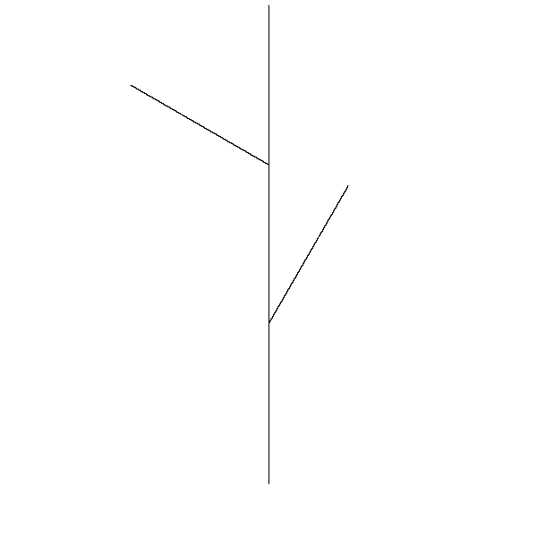
You can test your code by drawing the curve that results from any list of L-system commands that does not use offshoots. For example, evaluating

lcommands = make_lsystem_command(make_rotate_command(150), make_forward_command(), make_rotate_command(-120), make_forward_command())
curvelist = convert_lcommands_to_curvelist(lcommands)
c1 = connect_curves_evenly(curvelist)
c2 = translate(c1, 0.3, 0.7)
c3 = position_curve(c2, 0, 0.5)
draw_curve_points(c3, 10000)

We have provided the position_curve procedure to make it easier to fit fractals into the graphics window:

position_curve(curve, startx, starty) — evaluates to a curve that translates curve to start at (startx, starty) and scales it to fit into the graphics window maintaining the aspect ratio (the x and y dimensions are both scaled the same amount)

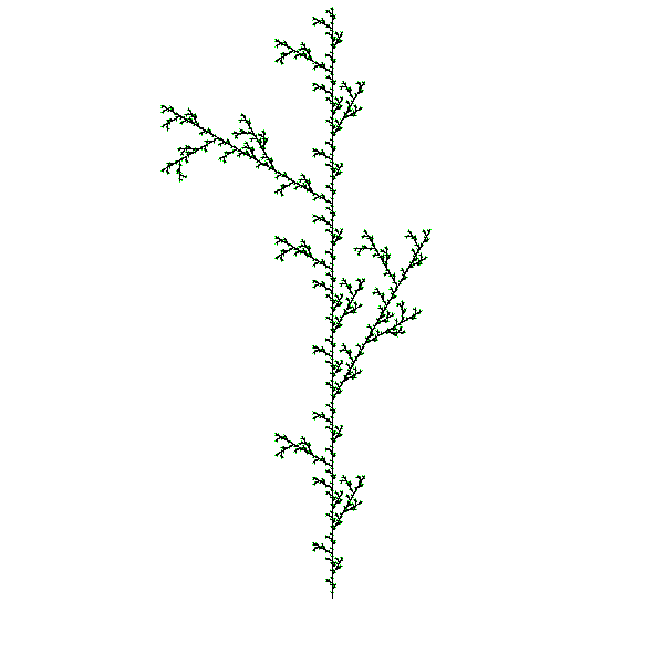
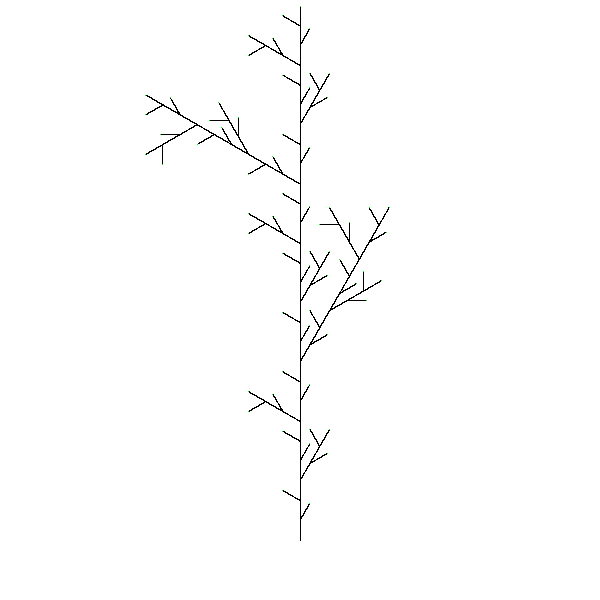
Now, you should be able to draw any l-system command list using position_curve and the convert_lcommands_to_curvelist function you completed in Questions 8 and 9. Try drawing a few simple L-system command lists before moving on to the next part. For example, given this input:

draw_curve_points(position_curve(connect_curves_evenly(convert_lcommands_to_curvelist(tree_commands)), 0.5, 0.1), 5000)

def make_tree_fractal(level):
	make_lsystem_fractal(tree_commands, \
          make_lsystem_command(make_forward_command), level)

def draw_lsystem_fractal(lcommands):
	draw_curve_points(position_curve(connect_curves_evenly( \
          convert_lcommands_to_curvelist(lcommands)), 0.5, 0.1), 50000)

For example, draw_lsystem_fractal(make_tree_fractal(3)) will create a tree fractal with 3 levels of branching.

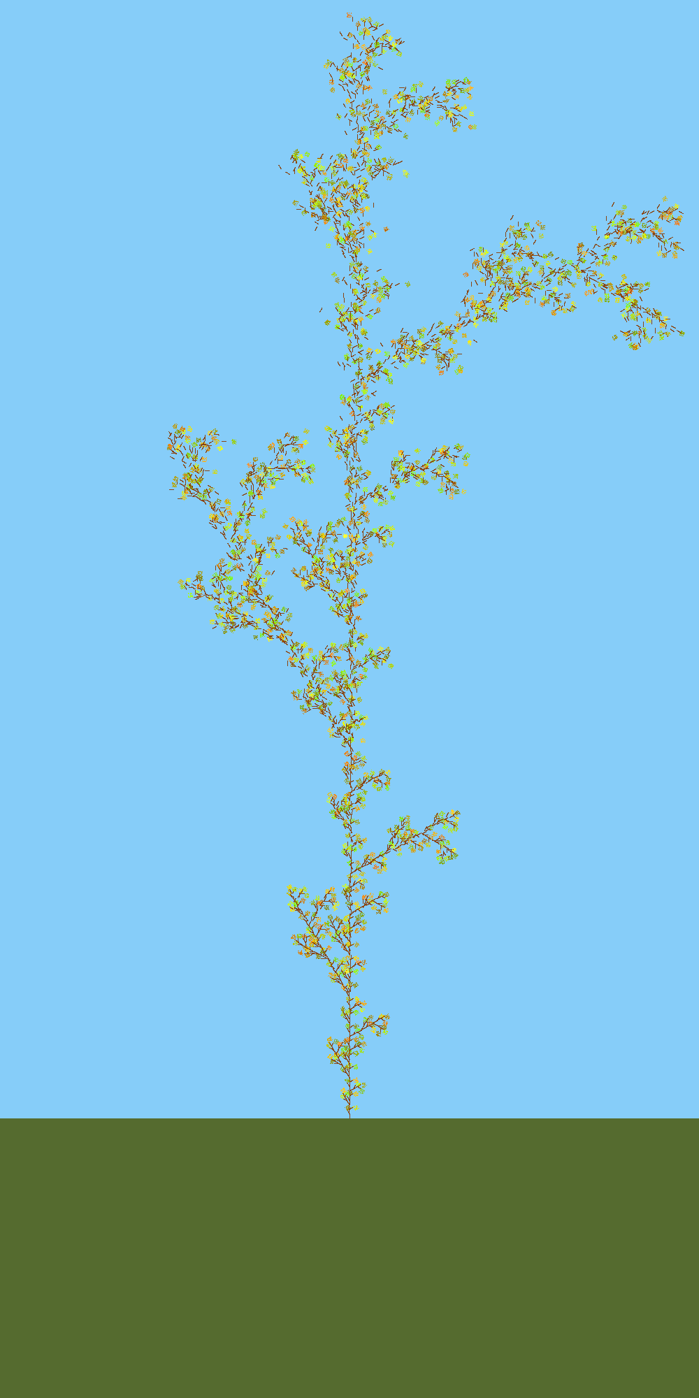
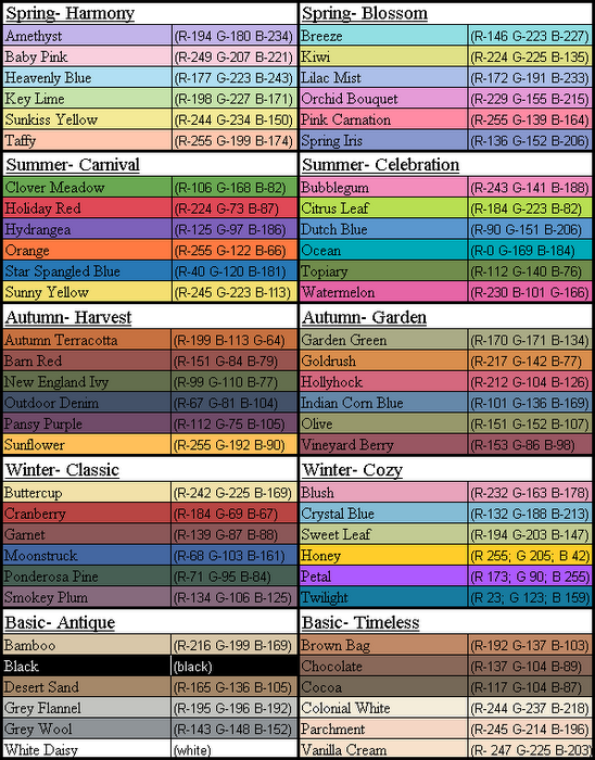
Draw some fractals by playing with the L-system commands. Try changing the rewrite rule, the starting commands, level and leaf curve (in convert_lcommands_to_curvelist) to draw an interesting fractal. You might want to make the branches colorful also (here's that color chart again). Try and make a fractal picture that will make a better course logo than the current Great Lambda Tree Of Infinite Knowledge and Ultimate Power.

Your last-displayed fractal image file is saved in fractal.svg in your current directory. It is over-written every time, so make sure that it looks right before you submit it!