1. Introduction
In the following few sections, Disjoint Support Decompositions (DSDs) will be discussed. This tutorial should prepare the reader for understanding the contributions of STACCATO and subsequently understanding how to use the STACCATO package. The tutorial will begin with a light intro on DSDs and will slowly add more material. The tutorial will then describe how DSDs can be created from BDDs. For a more technical/detailed understanding of DSDs, please consult the references at the bottom of the home page.
The figure below is a high-level diagram of a DSD. A function, F, can be written as F = K(A1,A2,A3...) where A1,A2,A3... are component functions whose support are disjoint. In the figure, F = K(J,x1,x2,...xj-1). Notice that the primary inputs for the component function, J, are disjoint from the other inputs of K. This property is necessarily true for DSDs.

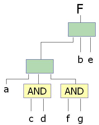
To better understand the concept of DSDs, consider the example below. This DSD represents the function F = a ((b XOR c) + d). As can be seen from the structure of the equation, an AND decomposition can be formed between the variable 'a' and the expression ((b XOR c) + d). However, it is possible to further decompose the expression producing a OR decomposition with (b XOR c) and d as inputs. By recursively checking for decompositions at each input an entire decomposition tree can be created. The following section will describe how this DSD is the only possible solution and that it is maximal.

1.1 Uniqueness of DSDs
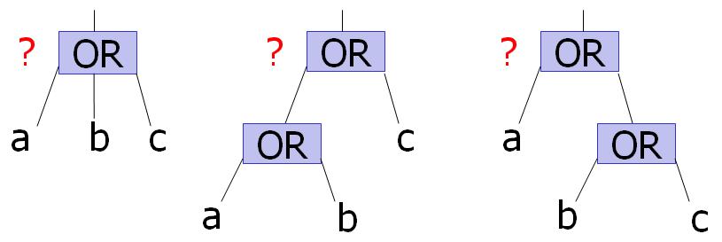
Ashenhurst showed that each function has a unique decomposition associated with it. However, Ashenhurst did not explain how to deal with associative operators like OR or AND. Consider, for instance, the simple function presented in the figure below--OR(a,b,c). How should this particular function be decomposed? Some of the possibilities are illustrated below.
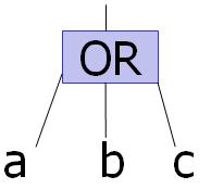
The solution to this problem is shown in the figure below. In general, the decomposition with the maximum amount of inputs is taken when considering an associative operator. By constructing DSDs with this constraint in mind, a unique, maximal decomposition can be formed for each function. In other words, only one maximal decomposition exists for each function.
1.2 DSD structure
The figure below provides a description of the decomposition tree structure as it occurs in packages that compute DSDs. In general, the DSD tree contains information on two different types of blocks, associative and prime. An associative block is an OR or XOR or AND block. A prime block is a 3-input or greater function that cannot be further decomposed. For instance, a mux function or a majority function would be considered prime blocks. The picture mentions something called a kernel function. A kernel function is one that relates the disjoint inputs of a certain block. For instance, the kernel of the function rooted at block F would be a function relating the disjoint inputs J1, x11, and J2. The kernel of the function rooted at block J2 would be a function relating the inputs x12, x13, x14. For discussion purposes, decomposition trees with a large number of internal blocks in their diagram will be classified as highly decomposable.

The decomposition tree structure also contains information on the type of data stored at each block. The type information provides the block type and the actuals list provides the list of immediate inputs to the block. Thus, the top block in the structure has the actuals list of J1, x11, and J2. Finally, the BDD pointer refers to the BDD rooted at that block that describes the function being decomposed. This BDD is necessary because, as we shall see shortly, an initial BDD of a function is needed to compute the DSD. The BDD is kept around mainly for indexing reasons for the unique table in the DSD package.
2. Constructing DSDs from BDDs
Different strategies for computing DSDs have existed for several decades. However, these solutions often required exponential amounts of work in the average case or involved inexact heuristic procedures. Recently, research has turned to computing DSDs from the BDD of a function (these works are referenced on the website homepage). An algorithm that requires polynomial complexity with respect to the size of the BDD was developed. Since, most representations of BDDs are polynomial in size compared to its support, this approach is very advantageous.
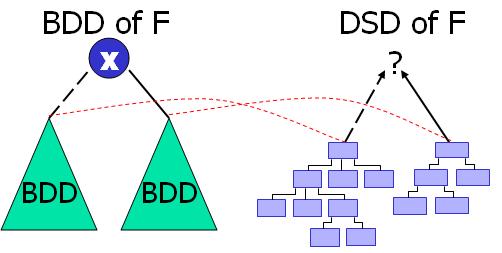
The figure above shows a high-level view of the procedure involved in constructing DSDs from BDDs. Looking at the picture, a BDD is represented as a top node with left and right children that form the then and else path for the BDD. This left and right child have corresponding DSDs. From these two decompositions, a new decomposition can be created that represents the entire function, F. This DSD is produced by applying several construction rules defined pretty thoroughly in Bertacco's thesis, listed in the references section. The DSD is produced by a bottom-up algorithm, requiring the decompositions of the BDD's children to compute the DSD of the BDD itself.
The next two sections will examine the two types of decompositions that are possible using this bottom-up approach. One is called an inherited decomposition because the decomposition of the parent is of the same form as one or both of its children. The second type is called new decompositions where a brand new decomposition is created based on the decompositions of its children. The following is meant to be a brief and intuitive introduction to both types of decomposition construction. A more technical and rigorous treatment of this material is provided in Bertacco '97.
2.1 Inherited Decompositions
An inherited decomposition is one where the decomposition of the left or the right cofactor of a function F is of the same structure as the decomposition of F. The algorithm in the Bertacco '97 paper outlines how to detect situations where a DSD of F can be obtained by inheriting it from either left or right cofactor with respect to a variable.
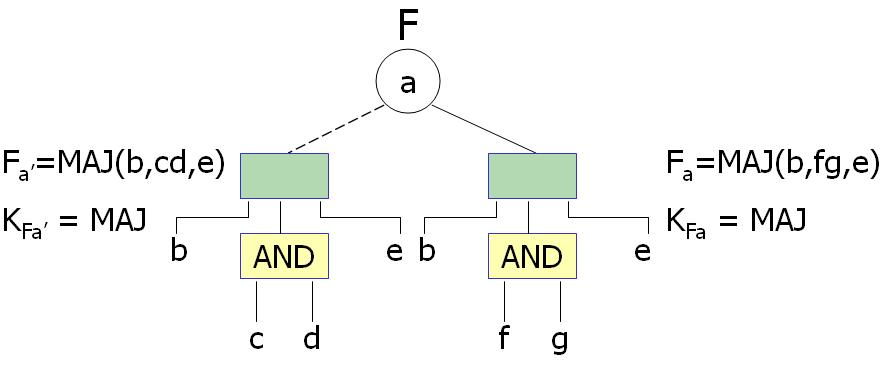
Consider the example above. The above figure defines the DSD for the functions, Fa=1 and Fa=0. The goal is to achieve the DSD of function F based on these cofactors. It turns out that in this particular example that the DSD of function F is an inherited decomposition. How is this determined? There are many techniques outlined in Bertacco '97 that explains how to determine this. For this particular case, the algorithm makes use of the fact that F(a=0,cd=1) == F(a=1,fg=1). In general, generalized cofactor operations are frequently required to identify a potential inherited decomposition.
How does knowing that the function, F, is an inherited decomposition produce the DSD of F. For this particular example, the DSD of F must be a decomposition that is a MAJORITY function sice both Fa=0 and Fa=1 are prime decompositions with MAJORITY function as the kernel. In order to construct the DSD of F, a majority function of disjoint inputs needs to be created. The result is the decomposition shown below.
2.2 New Decompositions
Sometimes there is no correlation between the DSD of the cofactors of function F and the DSD of F. Constructing the DSD of F in these situations requires the implementation of an algorithm defined in Bertacco '97 that identifies Common and Exclusive blocks between the left and right cofactors. A new prime decomposition is constructed with these blocks as members of its actuals list along with the top variable of the function F.
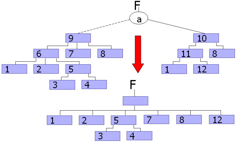
A high level depiction of this process is shown in the above figure. To make this picture as non-specific as possible, the blocks represent arbitrary decompositions where each subtree is disjoint from other subtrees is the larger tree (there is no reconvergence of primary inputs). Starting with the DSDs of the cofactors of function F with respect to variable a, we are able to obtain the DSD of the function F by identifying Exclusive and Common blocks. One can see that both DSDs of the cofactors contain blocks 8 and 1. These blocks are Common to both decomposition trees and will make up part of the actuals list for the new decomposition. Blocks 2, 5, 7 occur only in the left DSD and are thus Exclusive blocks and will also make up the actuals list for the new decomposition. Finally block 8 occurs only in the right DSD and is an Exclusive block that will also be added to the new actuals list. Notice that block 6 is not added as an Exclusive block because one of its inputs is not disjoint from the right DSD. Also notice that block 5 is taken instead of both 3 and 4 because block 5 dominates blocks 3 and 4 that are also Exclusive and the most dominant block is selected to form the new actuals list. The resulting new decomposition is a prime decomposition where the actuals list consist of these Common and Exclusive blocks and the variable a.